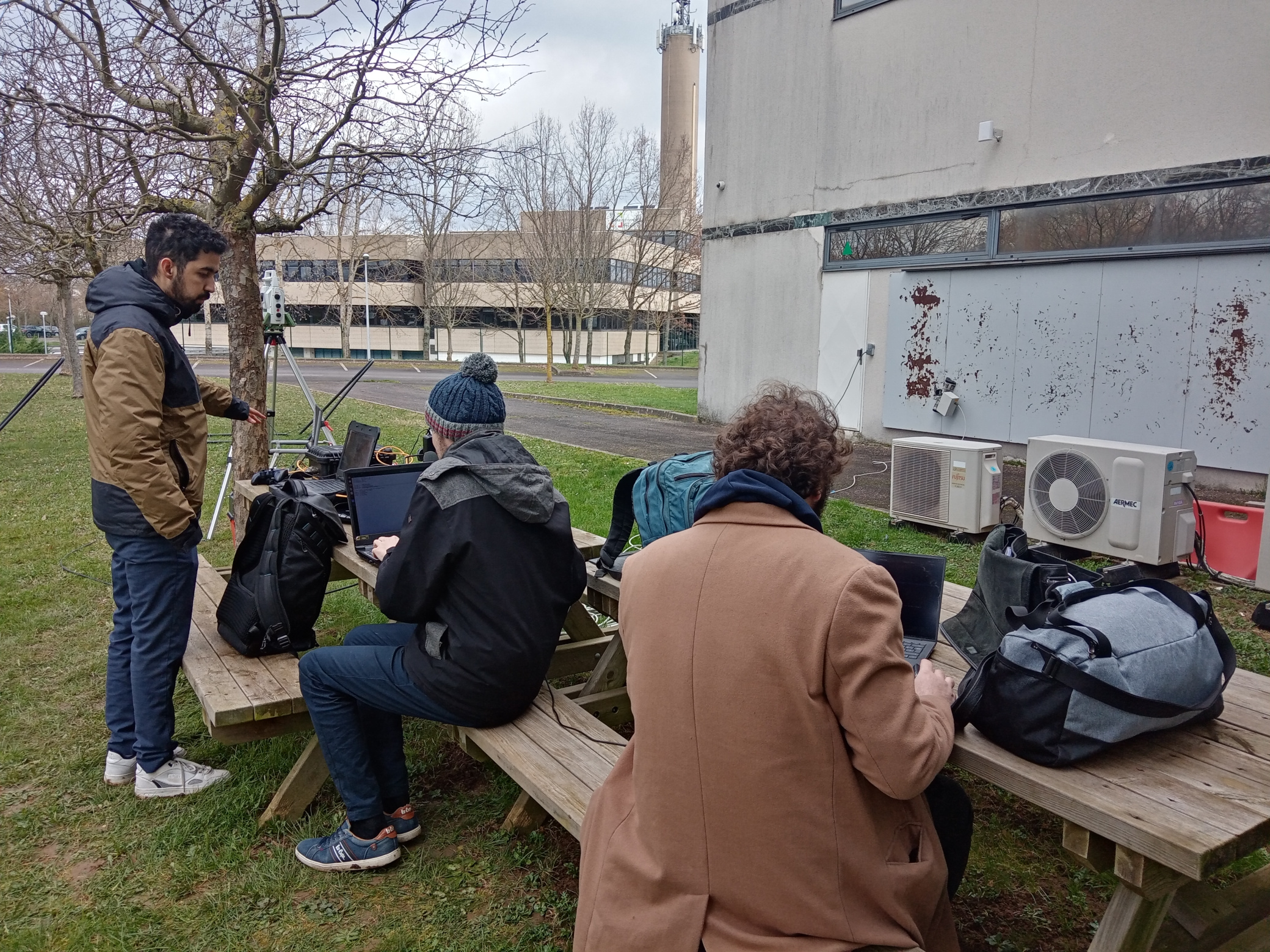
In February 2024, the INSA Lyon team met up with the CNRS’ team to work on a cooperation between real and simulated robot. Here’s their results:
1. Introduction
In robotics, there are many steps to develop an algorithm, a control command behaviour, studies, developing, test in simulation and test with real robot. This paper is placed between the last two. To pass form the simulation test to the real test we obviously need the same number of robot, but it is isn’t always the case. To pass thought, we want to do experiments with real and simulated robot at the same time. In this article we explain our work to do a cooperation between a real robot and simulated robots in the Gazebo software. On this project as robot we used crawler. A crawler robot is a ground robot like with a particularity which is it can move on a wall thank magnetic wheel (see Figure (a)). To allow his power supply, it connects by a cable from a base. So as it’s on a wall, if it moves on a cable of other crawler, it can fall. This issue is taking into account on the Path Planning.
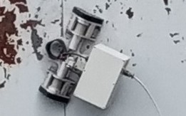
Figure 1(a) Real crawler on the metallic wall
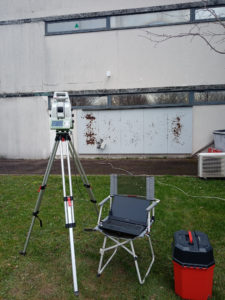
Figure 1(b) Real robot with the Leica platform
To know is relative position on the wall we used the Leica platform and markers. This platform detects the four markers put on each corner of the wall and one on the robot and send their position in the function of itself.
2. Path planning
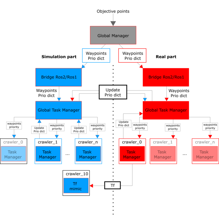
The mission is planned using the ROS2 node Global Manager (see Figure 2), which takes the objective points as input and outputs the paths to be followed by each of the robots and the order of priority at the corners of each obstacle. This node also manages the priority dictionary by sending the priority at a requested waypoints and by updating the dictionary when necessary. For this experiment, as the simulation and the real robot are on ROS1, a bridge had to be used. To minimise the amount of data crossing the bridge, we decided to create an ROS1 Global Task Manager node. This node retrieves the robot paths and the order of priority sent by the Global Manager and passes them on to the robot Task Managers. This node also manages the priority dictionary instead of the Global Manager. Initially, only one Global Task Manager was to be used. However, the Gazebo simulation necessarily uses simulation time for certain messages, whereas the real crawler uses global time, so we had to create two different ROS1 environments and therefore two Global Task Managers, as shown in Figure 2. This decision meant that we had to set up a system to enable the two Global Task Managers to communicate with each other in order to maintain consistency between the two priority dictionaries.
Figure 2: main logigram, (a) real part in red, (b) simulation part in blue, (c) unreal element of each part in transparency
3. Simulation software
To simulate an environment and robot model, we use gazebo, a robotic software. As the planning node does not differentiate between real and simulated crawlers, they must be defined in a common reference frame. The real one is defined by the Leica platform with the x axis is along its view axis. So the crawlers moved along the y/z axis, y being the horizontal axis and z vertical one, the simulated world must be defined on the same axes.
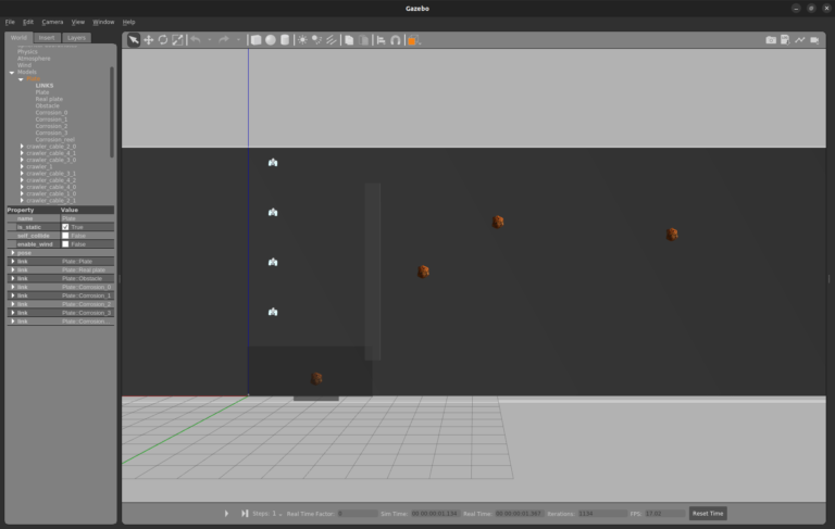
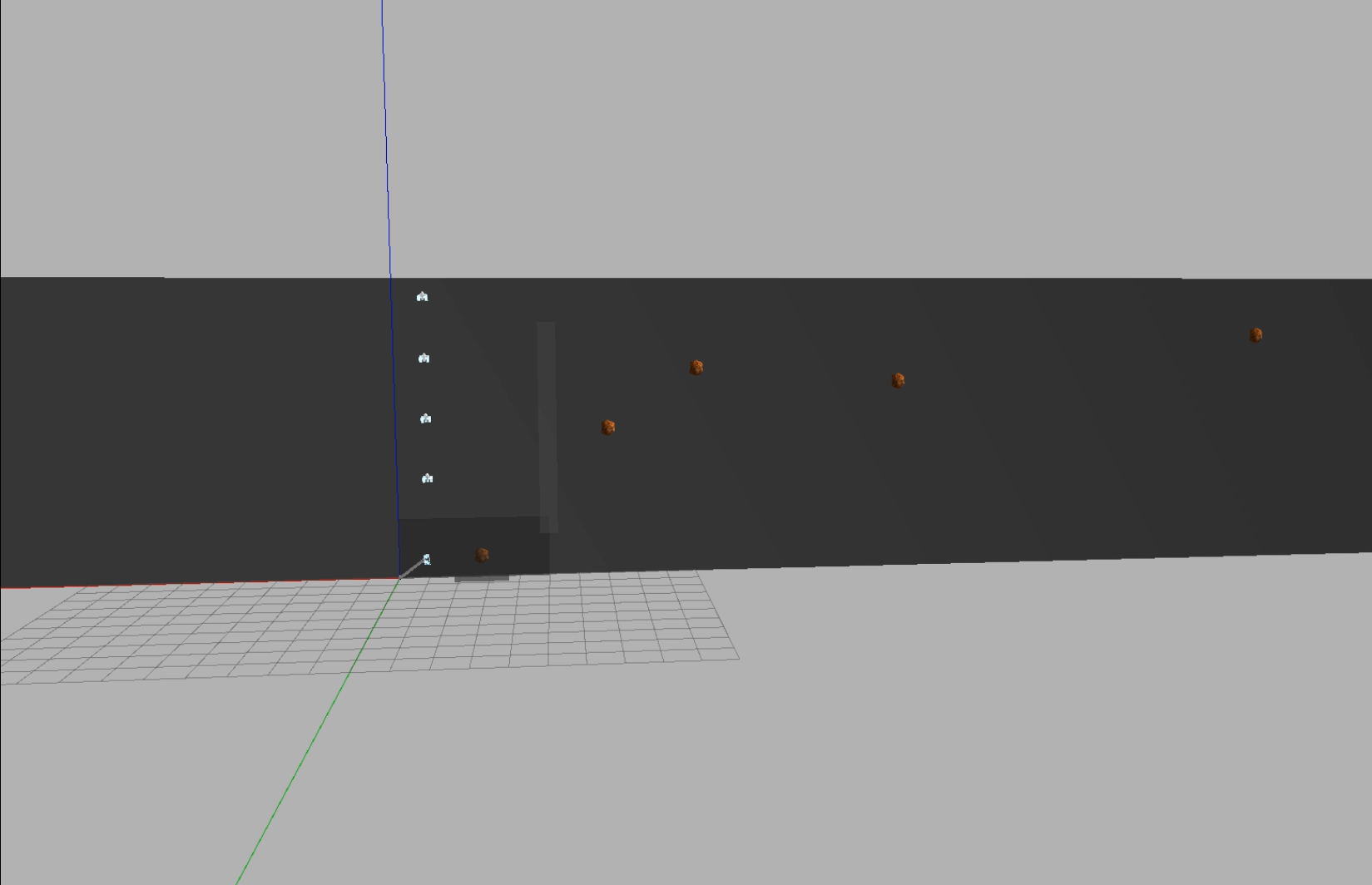
Figure 3: The simulation word with 4 simulated robot and one spectral robot
3.1 The world
The environment is defined by a world file with a 100×10 meter plate. On this plate we put some corrosion on each objective point to monitor if the crawlers reach their point. And, as we want to see the priority manage between crawlers we add an obstacle along the z axis defined by his four corner points as contact point.
3.1.1 Real plate on the simulation world
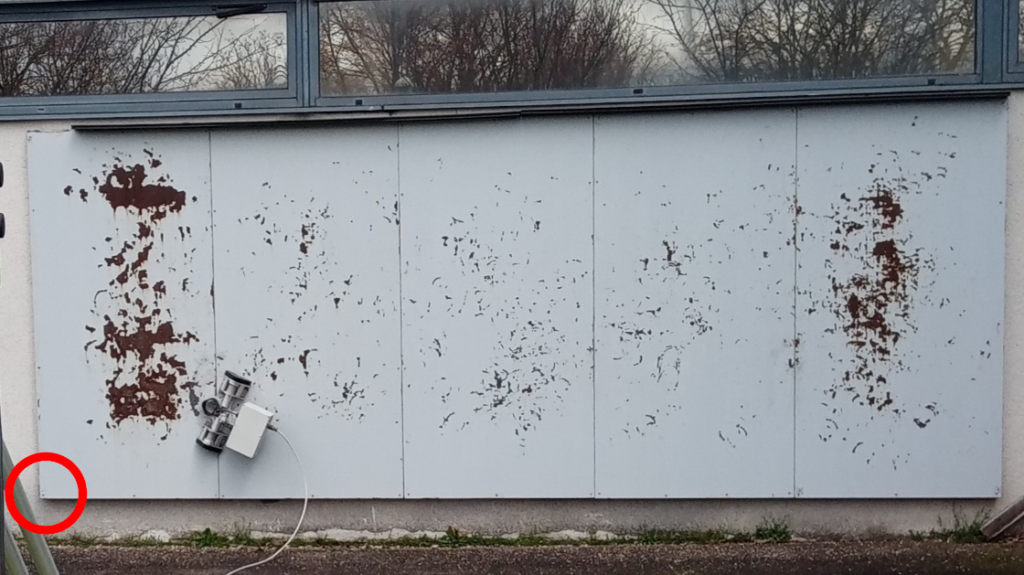
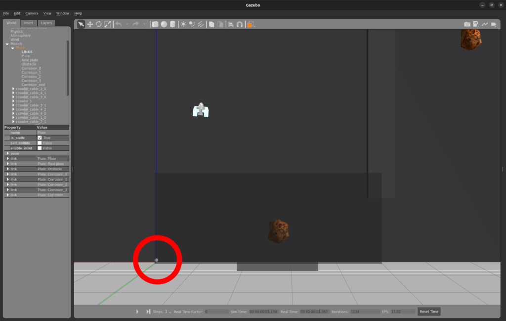
To see is real collaboration with the simulated robot, we need to see the real metallic plate in the simulation. For that, we add a transparent plate is origin is defined by the Leica platform on the bottom left of the plate Figure 4 (a)(The red circle corresponding to the origin of the plate). This simulated plate is the darkest one on the Figure 4(b). To simplify the experiment we place the simulated plate origin on the world frame.
Figure 4 (a) Real plate and the real crawler.
(b) The real plate into Gazebo.
So thank this origin, we know the pose of the real robot on the simulation. For the world creation, the only difficulty we had to overcome was that the gazebo world frame was not the same as that on Rviz. There is a rotation on the Z axis, so the x is -y and y is x.
3.2 The launch
To manage how many crawlers we want and with which control command node, we generate a launch file.
3.2.1 Crawlers
For this experiment, we want to do a collaboration between 5 crawlers. As we have only 1 real crawlers, we generated 4 crawlers with specific namespace from crawler 1 to crawler 4 in gazebo, the crawler 0 being the real crawler. Each crawler has two main nodes, one to manage the task and the second to do the task, together they are the task manager. This namespace allows to give the specific trajectory and command to the specific crawlers. To enable the planning algorithm to work, we create a fictive crawler 0 on the launch file with the same nodes as the others(see Figure 2) but he doesn’t have a model.
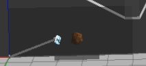
Figure 5: Real robot on the simulation
3.2.1.1 Real crawler on the simulation
As the crawler 0 haven’t nay model, we cannot see the displacement of the real crawler. For that, we add a model of crawler without task manager to mimic the real robot behaviour (see Figure 5). To prevent any problem with namespace, we named it crawler 10. Even if is number isn’t really important, it must have a name with an underscore followed by a number to allow the connection with its cables. As the pose of the real robot is defined by the Leica thank a prism on it, the frame of the crawler on the world isn’t its footprint. So in fact, the crawler in the simulation levitate. For more realistic effect, a new transformation must be done from the prism to its footprint.
3.2.2 Control command
For a better study of the collaboration between simulated and real robots, we make the same architecture of command (see Figure 6). At first, all crawler received there specific waypoints from the Global Task Manager (see Figure 2). After that, each crawler asks for the global manager, which have the dictionary of priority of all crawler, if it has the priority to reach the point. If the response is true, the crawler reaches the point and send to the global manager to update the priority list for the following crawler. If it hasn’t, the priority, the crawler waits until it has the priority. The main difference between the real crawler and the simulated one is the command to reach the point. But there is a little problem. As the crawler 0 on the simulation can reach any point because it hasn’t modelled. It can block the priority of a point. To prevent that, like we mentioned in 2. Path Planning, the dictionary was shared between the global task manager for the simulation and for the real part (see Figure 2).
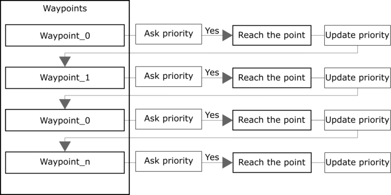
Figure 6: The architecture of the control command code for each crawler
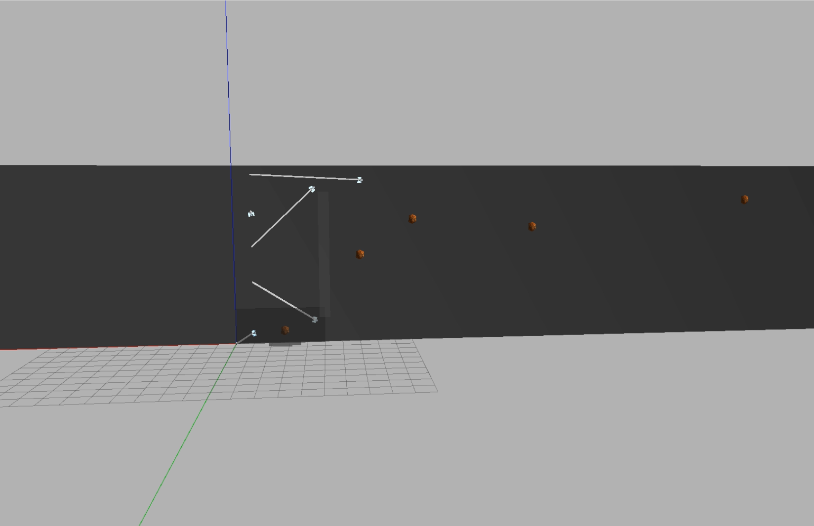
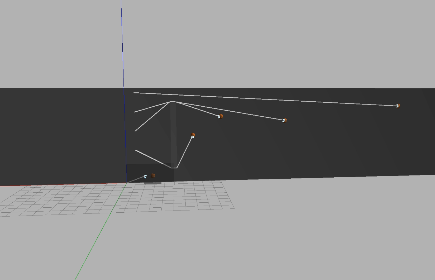
3.2.3 Cables
As we explain on the Introduction part, the crawler has to be connected to a cable to its power supply. To simulate these cables we add a pseudo robot arm which orients itself in a direction is targeted, at first the crawler position. Its length is computed by the Euclidean distance between the base and the crawler. When the cable touches an obstacle, here a rectangle defined by is four corners, it changes is target to the point of contact. Then a new cable spawns to the contact corner and orient itself to the crawler has its turn.
3.3 Conclusion
So to conclude, the simulation part was composed by a big metal plate along the y and z axis. On this plate there are all the target position as corrosion and a rectangle obstacle to visualise the priority management. And, in transparency there is the real plate. We put as many crawlers as we want. They must be named from crawler 0 to crawler (j-1) With j, the number of crawlers. In these crawler, all named from crawler 0 to crawler (i-1) is the real ones. And to simplify the allocation of namespace, we can say the spectral crawlers which mimic the real ones was named from crawler j to crawler (j+i-1) In the case of the experiment, i = 1 and j = 5.
4. Conclusion
To conclude all this experiment, we have experimented the architecture using pre-defined objective points, which have been ”hard-coded” in the Global Manager node. As a result, we manage to send the right paths to each of the robots and priorities are managed correctly. Unfortunately, for the time being, this can only be seen in the simulation because the real crawler did not function correctly during the experiments. However, the Task Manager of the real crawler did receive the correct path to follow. To go further, we want to test the interaction between simulated and real robot with more and other kind of robot like turtlebot. We also want to use only one global task manager to simplify the architecture of the code.